It’s very rare for both the underlying generative processes that produce the raw data, and the systems we use to measure, transform, and store that raw data, to be static and unchanging. More commonly, they evolve: distributions shift, relationships and constraints between the different dimensions of the data drift and break, data stops being available, and assumptions about the semantics of certain attributes cease to be valid. Multiple of those shifts can be happening on different timescales, and sometimes in abrupt ways.

This can have a profound effect on machine learning models. An underlying assumption of machine learning models is that the state of the world observed at training time is representative of the environment at which the model is deployed (typically, some time after training). When that assumption is invalid, in the best case scenario, predictive performance might be degraded; a monitoring component might be able to detect this regression, attribute it to a specific root cause, and trigger a retrain using a different dataset. In the worst case, it will continue to silently, happily serve non-sensical results.

Below, I wrote some notes about how concept drift is defined, how it is detected, and how ML systems can cope with it.

What is concept drift?

Concept drift is a shift in the relationship between covariates ($X$; the features used in the model) and the target variable ($y$; the variable being modeled). The “concept” in the name is the latent context that defined that relationship.

Concept drift can be characterized by comparing the joint distribution $p(X, y)$ of the test dataset, and assessing how much it changed compared to a reference dataset. It also encompasses data drift and label shift.

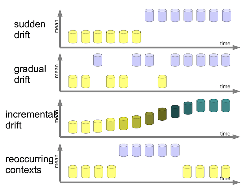
In ¹, concept drift encompasses:

• a sudden change in context, where the data changed abruptly due to discontinuous changes in the data generation mechanism;
• a gradual drift, where a new contexts is gradually introduced;
• an incremental drift, where the context smoothly transitions to a new baseline;
• a periodic drift, where a context might periodically be reintroduced.

In a supervised domain (where the label $y$ is known immediately, or close to), concept drift typically manifests itself in reduced predictive performance. More often, concept drift happens in an unsupervised domain: at inference time, once the model is deployed, we might have access to only a small subset of labels, or they are only captured after substantial latency. Because of that, the problem might not become apparent for some time; all the while, the model has been serving incorrect predictions due to concept drift.

Furthermore, the lack of labels presents an additional hurdle. Take a fraud detection problem: certain fraudulent behaviors might masquerade as benign by mimicking benign behavior observed in the train dataset. The features might not have changed, but the relationship of the model features and the (now latent) concept of fraud has.

Measuring concept drift

Distance between distributions

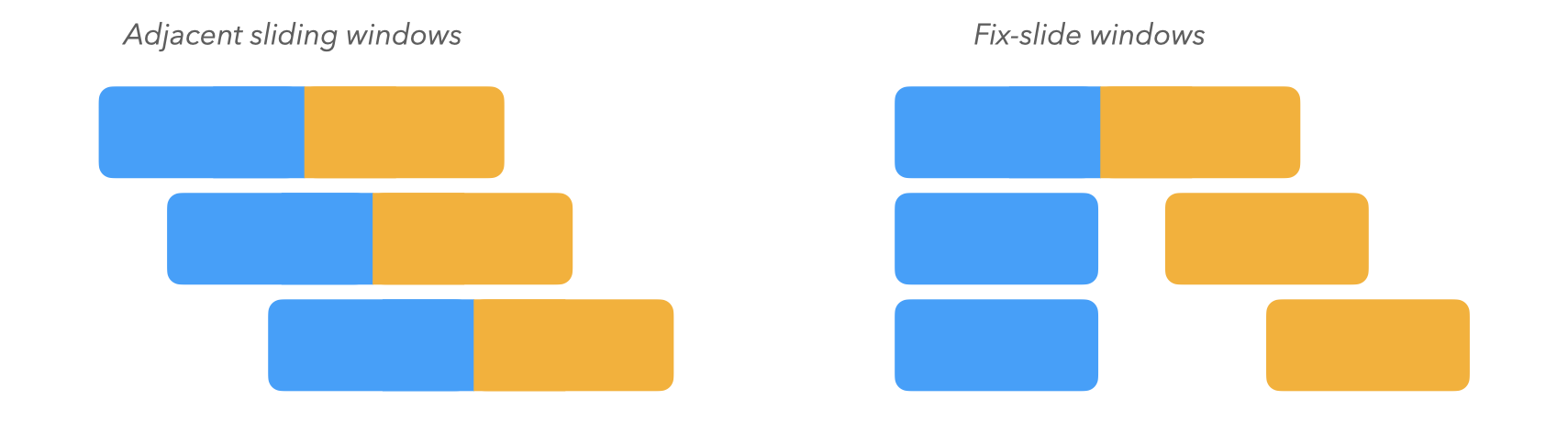
There are several techniques for measuring concept drift proposed in the literature. A typical heuristic consists of measuring the difference in the probability distribution of the data, as sampled within a reference window and a test window spanning a later time range. To fully capture different types of concept drift, a variety of window layouts and sizes should be selected. Adjacent sliding windows (where the reference and test windows are one after the other) measure recent, abrupt change, while fix-slide windows compare a fixed reference window and a sliding window, measuring longer-term drift.

² propose the Kullback-Leibler (KL) divergence to quantify the “distance” between the two distributions. Briefly, for two distributions $p$ and $q$, the KL-divergence measures the expectation value of the logarithmic difference between them, weighted by $p$:

Concretely, one could assign $p$ as the distribution of the variable(s) of interest within the reference window, and $q$ with the test window.

Things to note about the KL divergence:

• it is non-parametric;
• it is not symmetric between $p$ and $q$;
• it diverges to infinity when $p \neq 0, q = 0$, which can interpreted as “an event that was deemed as possible by $p$ is impossible per $q$, therefore these distributions are maximally different”.

In practice, the latter situation often happens when sampling a distribution from a finite dataset; in that case, one should smooth the distribution to account for unseen values. This is concretely done by adding “pseudocounts” to every bin.

In R, the entropy package implements the function KL.Dirichlet which computes the KL-divergence with added pseudocounts.

An alternative measure to the KL divergence is the Jensen-Shannon (JS) divergence. The JS divergence is a smoothed, symmetrized version of the KL divergence, defined as:

The JS divergence is bounded within $0 \leq JS \leq 1$, and does not diverge when one of the distributions is zero (or close to zero) and the other is non-zero.

It can be trivially implemented using the KL divergence formula:

library(entropy)

# Returns the empirical JS distance between two
# vectors of counts.
JS_empirical <- function(y1, y2) {
    f1 <- freqs.empirical(y1)
    f2 <- freqs.empirical(y2)
    fm <- 0.5 * (f1+f2)
    0.5 * (KL.plugin(f1, m, unit="log2") +
           KL.plugin(f2, m, unit="log2"))
}

Comparing performance of learners

Another option for detecting concept drift – if labels are available – is to keep track of performance metrics of models on unseen data, such as AUC/AUPR, F1, and Brier scores.

³ proposes a system that pairs two online learners: a stable learner $S$, trained on a growing window of data encompassing all the examples seen up to time $t$, and a reactive learner $R_w$ trained on a sliding window of fixed length $w$. The stable learner outperforms the reactive learner as long as the concept is constant, but will start mispredicting as the data transitions to a new concept. Since $R_w$ is trained on a smaller window, it can react more quickly and act as a lagging indicator of drift.

As a heuristic, the system keeps track of the number of incoming examples predicted correctly by $R_w$ and incorrectly by $S$; once that number passes a certain threshold, the training window of $S$ is clipped to be the same as $R$ before starting to grow again.

Taking action

Once a way to recognize concept drift has been established, a threshold should be chosen to establish the significance of the change, in order to distinguish actual drift from random noise.

When that bar is reached, and we conclude that concept drift is happening, a variety of automated strategies could be set up:

• retraining the model;
• reducing the size of the training data, to reduce the “inertia” of the model and respond more quickly to change;
• weighting recent samples more heavily;
• if the drift is known to be periodic, inducing that knowledge in the model. For instance, if a new cohort of customers is onboarded every three months, it can be helpful to include a time-dependent term in the model, or sample training examples from a longer baseline.

References

History of changes

• 04/09 - Added JS divergence, Bach et al. paper
• 04/06 - First revision