latex2exp: a package to render LaTeX in R graphics
This month, I pushed a big update to latex2exp, bumping it to version 0.9.
latex2exp is the R package for rendering LaTeX-formatted text in any plotting context. This package lets the user add formatted text (e.g. bold, italic, underline, different font sizes…), mathematical symbols, and equations to plots. Although this capability exists in base R, latex2exp makes it more accessible by exposing it via LaTeX, which is the most common standard for typesetting mathematical formulas.
The 0.9.3 update massively increased the number of LaTeX commands recognized, reworked the parser to work correctly in circumstances where the old parser would fail, improved documentation, and expanded its test suite to include a large number of sample expressions, seen-in-the-wild uses of latex2exp, and edge cases.
In this post, I will outline briefly about how latex2exp came to be, how it works, what changed and what the roadmap for the package looks like.
Typesetting formatted text and formulas in base R
The primary way to add formatted text and mathematical notation in base R is to use plotmath expressions.
plotmath
(described in ?plotmath) is a DSL that comprises
expressions that obey the syntax of regular R code, but are specially
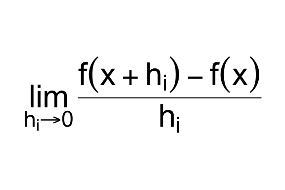
interpreted by a renderer. An expressions such as
expression(lim(frac(f(x+h[i])-f(x), h[i]), h[i] %->% 0))
combines function calls, subscripts, and operators like %->% to
produce a valid, unevaluated R expression. Each operand and token is
then interpreted by the renderer at plotting time; for instance, the
expression above is rendered as
 Plotmath expressions can be used as plot annotations, titles, axis and
legend labels in base R, lattice, and ggplot2 graphics.
Plotmath expressions can be used as plot annotations, titles, axis and
legend labels in base R, lattice, and ggplot2 graphics.
This system has a number of disadvantages:
- The syntax is unfamiliar to most R users LaTeX is the de-facto standard for typesetting mathematical equations. Although the plotmath system is somewhat reminiscent of LaTeX, anecdotally, new and experienced R users find the plotmath syntax unnecessarily different and complicated. While it is an interesting application of R’s ability to do metaprogramming, in practice, this DSL does not bring tangible advantages over a string containing LaTeX notation.
- Equations have to be valid R syntax. Because a plotmath
expression has to be parsable, a number of equations need
workarounds in order to be written as valid R expressions. Those
equations typically need workarounds combining
{}(braces are invisible groups),phantom()(an invisible token) and*(which juxtaposes the operands).
For example, the equation a < b < c is not valid R code; the correct
way to typeset the equation would be
expression({a < b} * {phantom() < c}). 3. It is not easily
extensible. As far as I can tell, there are no hooks for introducing
new symbols and functions. 4. The quality of the output is… not
ideal. Compared to a full LaTeX typesetter, the rendered output is
merely passable. Limitations include the inability to italicize symbols
and greek letters; typeset and align multi-line equations; and, in some
cases, properly resize symbols in presence of equations containing tall
elements, resulting in artifacts.
latex2exp tries to address (1)-(3) by providing an easier-to-use interface to plotmath’s capabilities. Because it is just a translational layer on plotmath, it cannot improve on the quality of the typesetting, although in many situations it can produce a higher-quality plotmath representation than a hand-written expression.
An interactive demo
Here’s an interactive demo! Enter a LaTeX expression into the text box on the right panel to preview how latex2exp will render it.
How latex2exp works
latex2exp, via its main function latex2exp::TeX(), parses an input
LaTeX string and tries to convert it to a plotmath expression. It does
that by scanning the LaTeX string looking for various types of tokens,
and translating them into the plotmath representation that is visually
closest to the ideal rendering.
For some expressions, the translation is straightforward. For example,
TeX(r"(\alpha)")
# is equivalent to
expression(alpha)
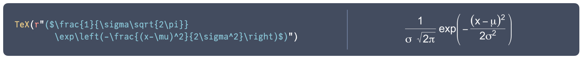
For others, the translation is not so straightforward, and latex2exp translates the LaTeX string into the closest equivalent, which might be a relatively complicated plotmath expression:
TeX(r"($\frac{ih}{2\pi} \frac{d}{dt} \ket{\Psi(t)} = \hat{H}\ket{\Psi(t)}$)")
# is equivalent to
expression(
  frac(ih, 2*pi) * phantom(.) *
  frac(d, dt) * phantom(.) *
  group('|', Psi(t), rangle) ==
  hat(H) * group('|', Psi(t), rangle))
)
A common source of bugs for new users of latex2exp is that the backslash
character inside strings is used to start an escape sequence, such as
\n (newline), \t (tabs), or \unnnn (a Unicode character). So, a
user attempting to write a TeX string such as "\Psi" will be greeted
by the error
Error: '\P' is an unrecognized escape in character string starting ""\P"
Prior to R 4.0, the only available option was to escape the backslash
character using a double-backslash, e.g. "\\Psi", a surprising first
hurdle for new users of latex2exp.
As of R 4.0, it is possible to use unquoted backslashes in a string, if
the string is marked as a raw string, e.g. r"(\Psi)". Raw strings
are written as r"(...)" with ... being any character sequence (see
?Quotes for a description of raw strings). I recommend using raw
strings when using the package (unless using R > 4.0 is not possible).
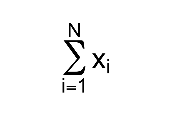
At any point, it is possible to obtain a quick preview of the output of
the call to TeX by calling plot() on the returned value:
e <- TeX(r"($\sum_{i=1}^{N} x_i$)")
plot(e, cex=3)
Finally, the package website has a filterable
table
of supported LaTeX commands and a preview of how they will be rendered.
The same table can also be invoked anytime from the R prompt using the
command latex2exp_supported().
What’s next?
As far as I can tell, the current version (0.9.3) of latex2exp supports all the LaTeX commands that can be feasibly rendered via plotmath (and a few more are “emulated” using some trickery).
The goal for the 1.x branch of latex2exp is to improve on workflows that are unnecessarily error prone, add new features that are hard or impossible to achieve with plotmath, and extend the range of examples provided in the documentation.
Specialized annotation geoms for ggplot and ggrepel
I would like to support ggplot more directly. Currently, for ggplot
geoms like geom_text, geom_label, and annotate that take a label
aesthetic, the input vector for the label aesthetic is expected to be of
type character, rather than of type expression. In order to plot
formatted text and formulas, the user is expected to pass a character
representation of the plotmath expression and remember to specify the
parameter parse=TRUE to force parsing of the expression.
This means that in order to use TeX with these functions, it is
necessary to use the parameter TeX(..., output="character") to force
it to return the character representation of the expression:
ggplot(mtcars, aes(x = wt, y = mpg)) + geom_point() +
  annotate("text", x = 4, y = 25,
           label = TeX(r"(\alpha+\beta)", output="character"),
           parse=TRUE)
This is unintuitive, error-prone, and unnecessarily verbose.
I propose to add the functions: geom_text_TeX, geom_label_TeX, and
annotate_TeX. These functions will forward to the underlying ggplot
functions, and set the appropriate parameters for the user, such that:
ggplot(mtcars, aes(x = wt, y = mpg)) + geom_point() +
annotate_TeX(x = 4, y = 25, label = r"(\alpha+\beta)")
will automatically parse the TeX input, turn it into an expression, and
forward it to annotate with parse=TRUE.
Multi-line equations
There is currently no way to introduce a line break in an equation.
I can see two possibilities for achieving this in a future 1.x version:
- Break the expression into separate labels, each containining a line of equation, and compute positioning coordinates that achieve the correct layout and alignment;
- Or, exploiting an undocumented (as far as I know) behavior of
plotmath, it appears to be possible to liberal use of the
atop()plotmath function to stack multiple equations on top of each other, wrapped in a call todisplaysize()to ensure each line is displayed with the correct font size.
The latter produces a passable-in-a-pinch output where each line is
center-aligned: 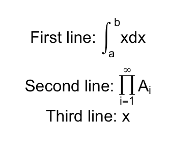
Gallery of examples
I am accumulating a few examples of usages of latex2exp – both from my own work, and in the wild – that can be used to showcase what the package can do for publication-quality plots.